
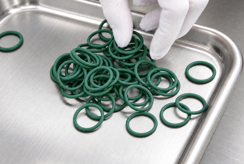
One of the most difficult questions in rubber engineering is also one of the most practical: how can the performance of a silicone O-ring over ten or twenty years at service temperature be estimated without waiting ten or twenty years for the answer?
Direct aging for the full service period is usually impossible during product development. Time-temperature superposition, commonly abbreviated as TTS, provides a way to extend the useful time range of laboratory measurements. Its central idea is that the same viscoelastic relaxation process can occur quickly at a higher temperature and slowly at a lower temperature. If temperature changes the rate of molecular motion without changing the governing mechanism, short high-temperature measurements can be shifted along the time axis to represent longer behavior at a selected reference temperature.
For a silicone O-ring, the useful output is not a claim that the rubber will simply “last for decades.” A defensible study predicts a defined property, such as compression stress relaxation, sealing-force retention, creep compliance, or modulus, and compares that prediction with a functional failure criterion. Fluid compatibility, groove geometry, pressure, movement, thermal cycling, and manufacturing variation must still be evaluated separately.
One Relaxation Process Viewed Two Ways
Silicone rubber is viscoelastic. Its response depends not only on load and deformation but also on the time available for polymer chains and network segments to move.
At low temperature or over a short observation time, molecular motion is relatively slow. Chain segments can make only limited local adjustments, so the material appears stiffer and retains more of its initial stress. At a higher temperature or over a longer observation time, the segments have more thermal energy and can overcome internal resistance more quickly. Stress relaxes faster, creep develops further, and the measured modulus decreases sooner.
This leads to the basic TTS relationship:
A short-time response at a higher temperature may represent the same stage of a relaxation process as a long-time response at a lower temperature.
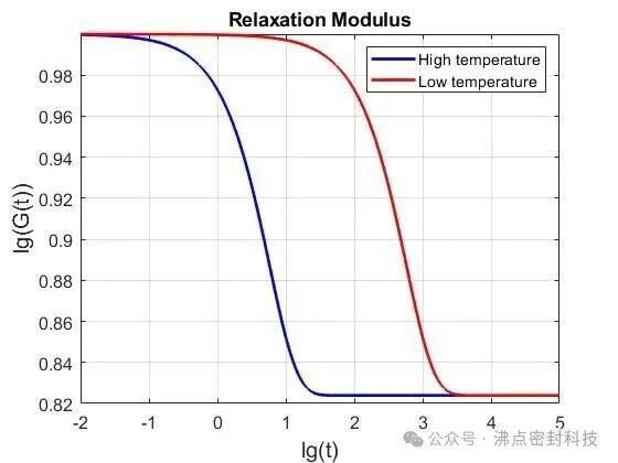
The important condition is that temperature changes the rate of the process, not its nature. When this condition is satisfied, the relaxation spectrum moves along the logarithmic time scale while retaining approximately the same shape. The material is then described as thermorheologically simple within that temperature and time range.
This distinction matters for O-rings. If the only important change is physical stress relaxation in an otherwise stable crosslinked network, horizontal shifting may work well. If elevated temperature also causes post-curing, oxidation, chain scission, volatilization, swelling, or a change in filler–polymer interaction, the high-temperature specimen is no longer following the same process at a faster rate. A simple time shift can then give a misleading life estimate.
Shift Factor and Reduced Time
The horizontal movement needed to align data from temperature (T) with data at the reference temperature (T_{ref}) is described by the shift factor (a_T).
Using the common relaxation-time convention:
aT = τ(T) / τ(Tref)
where (τ(T)) is the characteristic relaxation time at the test temperature and (τ(T_{ref})) is the corresponding relaxation time at the reference temperature.
The equivalent time at the reference temperature is then:
tref = tT / aT
For a test temperature above the reference temperature, relaxation normally occurs faster, so (a_T) is less than one. If (a_T = 0.01), one hour at the higher temperature corresponds to 100 hours at the reference temperature. Some reports instead use an acceleration factor (AF = 1/a_T). Under that convention, the same example is written as (AF = 100). The report must state which convention is used because reversing the factor changes the prediction by orders of magnitude.
Building a Master Curve
The laboratory procedure is conceptually simple:
- Select one measurable response, such as compression stress relaxation at a fixed O-ring squeeze.
- Test equivalent specimens at several controlled temperatures.
- Plot each response against logarithmic time.
- Choose a reference temperature that represents the intended service condition.
- Shift the other curves horizontally until their overlapping regions agree.
- Fit the resulting shift factors as a function of temperature.
- Join the shifted data into a master curve at the reference temperature.
The master curve may cover a much wider time range than any individual test. The overlap between adjacent temperatures is essential. A visually smooth curve produced without enough shared data can hide an incorrect shift or a change in mechanism.
For O-rings, compression stress relaxation is often more directly connected to sealing than an unloaded tensile modulus. The specimen should remain at a defined squeeze in a fixture that represents the relevant loading mode. Force is recorded over time, and the retained-force ratio can be expressed as:
R(t) = F(t) / F0
where (F_0) is the initial compressive force after the agreed seating period and (F(t)) is the force after time (t). A project-specific limit, such as the minimum retained force required to maintain leakage control, can then be placed on the master curve.
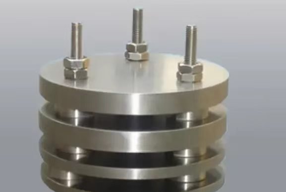
Compression set data can support compound screening, but it is not interchangeable with stress relaxation. Compression set testing measures dimensional recovery after unloading, whereas stress relaxation measures the loss of sealing force while compression remains applied. A long-term sealing prediction should use the response that is most closely tied to the actual failure mode.
WLF and Arrhenius Shift Models
After experimental shift factors have been obtained, a mathematical model is used to describe how (a_T) changes with temperature. The two most common models are the Williams–Landel–Ferry equation and the Arrhenius equation.
WLF Equation
The WLF form is commonly written as:
log10(aT) = −C1(T − Tref) / [C2 + (T − Tref)]
The WLF model describes the strong change in relaxation time associated with free-volume changes near the glass-transition region of an amorphous polymer. Increasing temperature increases molecular mobility, allowing relaxation to proceed more quickly.
When the reference temperature is the glass-transition temperature (T_g), the often-quoted universal constants are approximately (C_1 = 17.44) and (C_2 = 51.6) K. These constants are useful as a reference, not as automatic silicone-compound values. Compound formulation, crosslink density, fillers, plasticizers, and the selected reference temperature can change the fitted constants.
WLF is generally considered over a range beginning above (T_g) and extending roughly toward (T_g + 100) K, provided one relaxation mechanism remains dominant. Silicone O-rings normally operate far above the very low (T_g) of silicone rubber. For long-term service-temperature predictions, an Arrhenius relation is therefore often more practical, but model selection should be based on the measured shift factors rather than the material name alone.
Arrhenius Equation
The Arrhenius relationship can be written as:
ln(aT) = (Ea/R) × (1/T − 1/Tref)
where (E_a) is the apparent activation energy, (R) is the gas constant, and temperatures are expressed in kelvin.
This model represents a rate process that must overcome an approximately constant activation-energy barrier. A plot of ln(a_T) against 1/T should be approximately linear over a valid single-mechanism range. Arrhenius shifting is frequently used for rubbery-state relaxation and for accelerated thermal-aging data, but the activation energy fitted for physical stress relaxation should not automatically be applied to oxidation or another chemical degradation process.
How the Model Is Selected
Model selection should not be reduced to whether (a_T) is “linear with temperature.” The practical sequence is:
- Obtain shift factors from curve overlap rather than assuming them in advance.
- Fit both physically plausible models over the measured temperature range.
- Compare residuals and check whether the shifted curves retain the same shape.
- Look for slope changes that indicate a transition in the controlling mechanism.
- Confirm that the fitted model predicts withheld test data before using it for long extrapolation.
If a single horizontal shift cannot align the complete curve, the material may require vertical shifting, separate mechanisms, or a different model. In that situation, a single master curve should not be forced through the data.
A Practical O-Ring Life-Prediction Workflow
A useful TTS program begins with the seal and its failure definition, not with the equation.
1. Define the Service Condition
Record the O-ring material, hardness, cure system, post-cure, dimensions, groove geometry, squeeze, gland fill, pressure, medium, temperature profile, movement, and target life. A constant 80°C dry-air application is not equivalent to an O-ring cycling between room temperature and 80°C in oil.
If the O-ring contacts a liquid, first establish that the compound remains chemically compatible. Swelling, extraction, hardening, or softening can change the relaxation response. Fluid immersion testing provides useful material-screening data, but combined heat, compression, and media exposure may still be required.
2. Define the Predicted Property and Failure Limit
Examples include:
- Retained compressive force at a fixed squeeze
- Creep compliance under a defined load
- Dynamic modulus at a specified frequency
- Leakage rate after thermal aging
- Compression set after a defined recovery period
The end-of-life limit must be linked to function. “Fifty percent stress retention” is not a universal O-ring failure point. One groove may maintain sufficient contact pressure at that level, while another may leak earlier because of pressure, tolerances, surface condition, or joint movement.
3. Select Temperatures Without Changing the Mechanism
Use enough temperatures to create overlapping time windows and reveal curvature in the shift-factor relationship. The highest temperature should accelerate the intended mechanism without introducing post-cure, oxidation, thermal decomposition, or a different phase or interface response.
For silicone rubber, choosing the highest temperature only from a generic heat-resistance statement is unsafe. The actual compound, pigment, filler, cure state, oxygen availability, specimen thickness, and medium all affect the usable acceleration range.
4. Control Specimens and Fixtures
Specimens should come from traceable production material and should represent the intended cure and post-cure condition. Compression fixtures need controlled spacer height, parallel loading surfaces, stable materials, and a documented squeeze. Force sensors and temperature chambers should be calibrated for the measurement range.
Replicates are needed because rubber properties and molded dimensions vary. The study should report individual results or statistical spread rather than only one smooth average curve.
5. Construct and Validate the Master Curve
Shift adjacent curves using their common regions. Record every shift factor, fitting range, and excluded point. Then test at least one additional temperature or duration that was not used to build the model. Agreement with this independent result provides more confidence than a high fitting coefficient alone.
6. Convert the Curve Into a Service-Life Estimate
Locate the defined failure threshold on the master curve and read the corresponding time at the reference temperature. Report the estimate with its assumptions, confidence interval or uncertainty range, and the maximum extrapolation beyond measured time.
The result should be written as a conditional prediction, for example:
Under dry-air exposure, constant 20% squeeze, and the tested compound and cure condition, the model predicts that compressive force will remain above the specified limit for the stated time at the reference temperature.
This wording identifies what was predicted and prevents the number from being reused for a different fluid, groove, temperature cycle, or compound.
Two Boundaries That Control Reliability
Boundary 1: TTS Requires the Same Dominant Mechanism
Simple time-temperature superposition is most reliable for a stable physical relaxation process. Long high-temperature exposure can add chemical change. Oxidation may break chains, additional curing may increase crosslink density, and volatile loss may harden the compound. These changes alter curve shape rather than merely moving the curve horizontally.
Useful checks include:
- Periodic unloading and reloading to separate recoverable relaxation from permanent change
- Hardness, mass, volume, and tensile measurements before and after aging
- Dynamic mechanical analysis to obtain independent shift factors
- Visual and microscopic inspection for cracking, tackiness, or surface change
- Comparison of curves in air, low-oxygen conditions, and the actual service medium when relevant
If post-aging modulus or hardness changes systematically with exposure, the study may be measuring both relaxation and chemical aging. Separate models or a more complete degradation study may be required.
Boundary 2: Extrapolation Is Not Unlimited
Every decade added beyond the measured window amplifies uncertainty in the shift factors, model constants, and failure criterion. A practical engineering rule is to avoid extrapolation far beyond the validated range; two to three orders of magnitude beyond measured time is sometimes used as a working limit, but it is not a universal guarantee.
Longer predictions require stronger evidence: more temperature levels, longer tests, mechanism checks, replicate data, independent validation points, and conservative acceptance limits. A mathematically smooth line cannot replace missing physical validation.
What TTS Can and Cannot Predict
TTS can extend a measured viscoelastic response and help compare compounds or process conditions. It is especially valuable for stress relaxation, creep, and modulus when the same molecular mechanism remains active across the test range.
It cannot independently account for every O-ring failure mode. A complete sealing-life assessment may also need to address:
- Fluid-induced swelling, extraction, or hydrolysis
- Thermal oxidation and ozone exposure
- Extrusion at pressure and elevated temperature
- Abrasion and friction in dynamic service
- Pressure and temperature cycling
- Groove tolerances and thermal expansion
- Installation damage, twisting, and contamination
- Production variation between material and molding batches
The master curve is therefore one part of a validation chain. Material screening, O-ring groove design, compression testing, media compatibility, dimensional inspection, and functional leakage testing should support the final decision.
Conclusion
Time-temperature superposition turns an unaffordable waiting problem into a controlled laboratory study. The same relaxation process is measured at several temperatures, represented by shift factors, assembled into a master curve, and fitted with a WLF or Arrhenius relationship appropriate to the observed mechanism.
For silicone O-rings, the most useful prediction is usually not an abstract material lifetime. It is the time required for a defined sealing-related property to reach a project-specific limit under stated conditions. That prediction is credible only when the curves superpose, the model is validated, chemical aging is excluded or separately modeled, and extrapolation remains controlled.
Understanding where TTS fails is as important as understanding how it works. That boundary is what turns a convenient equation into an engineering method.
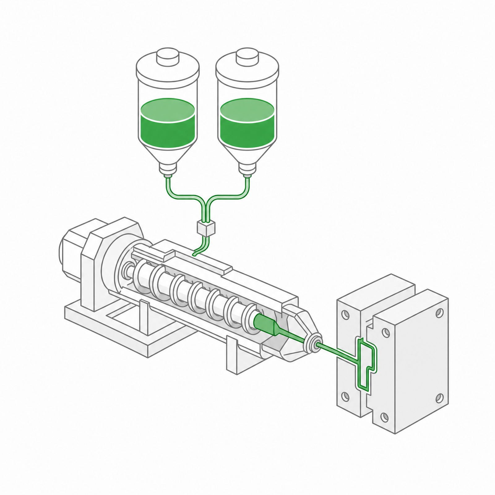 LSR Injection Molding
 Silicone Rubber Overmolding
 Compression Molding
 Silicone Rubber Extrusion
 In-house Tooling